How to Use Conditional Formatting in Google Sheets
Conditional formatting adds selective formatting to your spreadsheet, so it’s easier to visually scan. Learn how in this tutorial.
![[Featured Image] A businessperson working on a spreadsheet on their computer while a coworker looks on.](https://d3njjcbhbojbot.cloudfront.net/api/utilities/v1/imageproxy/https://images.ctfassets.net/wp1lcwdav1p1/5JCxu2o1GNer80SGNTxqHn/9968ac588b4c7ec8fe034b78becef805/GettyImages-1401958744.jpg?w=1500&h=680&q=60&fit=fill&f=faces&fm=jpg&fl=progressive&auto=format%2Ccompress&dpr=1&w=1000)
Key takeaways
When sifting through a large data set in Google Sheets, you may find it useful to add color or other formatting to visually identify certain information.
Conditional formatting automatically formats cells with color or text styling if they meet a predefined criterion, or rule, set by the user.
To use conditional formatting, access Format in the Google Sheets menu, select Conditional formatting, choose your preferred color, and apply the formatting rules and style.
You can use 19 different rules within single-color conditional formatting in Google Sheets.
Learn how to apply conditional formatting in Google Sheets and troubleshoot common errors.
How to do conditional formatting in Google Sheets
Here's a quick summary of the steps you'll take to apply conditional formatting in Google Sheets:
Select the range you want to format.
Go to Format in the top menu. Select Conditional formatting.
Select either Single color or Color scale.
Apply a formatting rule (or rules) and a formatting style.
Click Done.
Let's take a closer look at each step.
What is conditional formatting in Google Sheets? Get ready to deepen your knowledge
To begin, you'll need your tab open to your spreadsheet. If you’re not already working with your own data set and want to follow along with our examples, make a copy of this template to practice.

1. Select the range you want to format.
The first step is to select the data range you would like to format. A range can consist of a single cell or multiple adjacent cells.
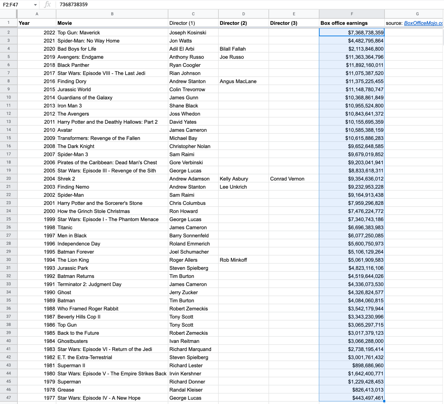
To select your range, click the first cell (top-left) in the range, hold the Shift key, then click the last cell (bottom-right) in the range. Alternatively, you can click the first cell in your range and drag your cursor to the last cell of your range. Your range is now highlighted. In the example below, the range in column F (“Box office earnings”) is highlighted, so the financial data contained within it can be selected for conditional formatting. Note that the highlighted range is also displayed in the upper left corner of the sheet, where “F2:F47” is displayed.
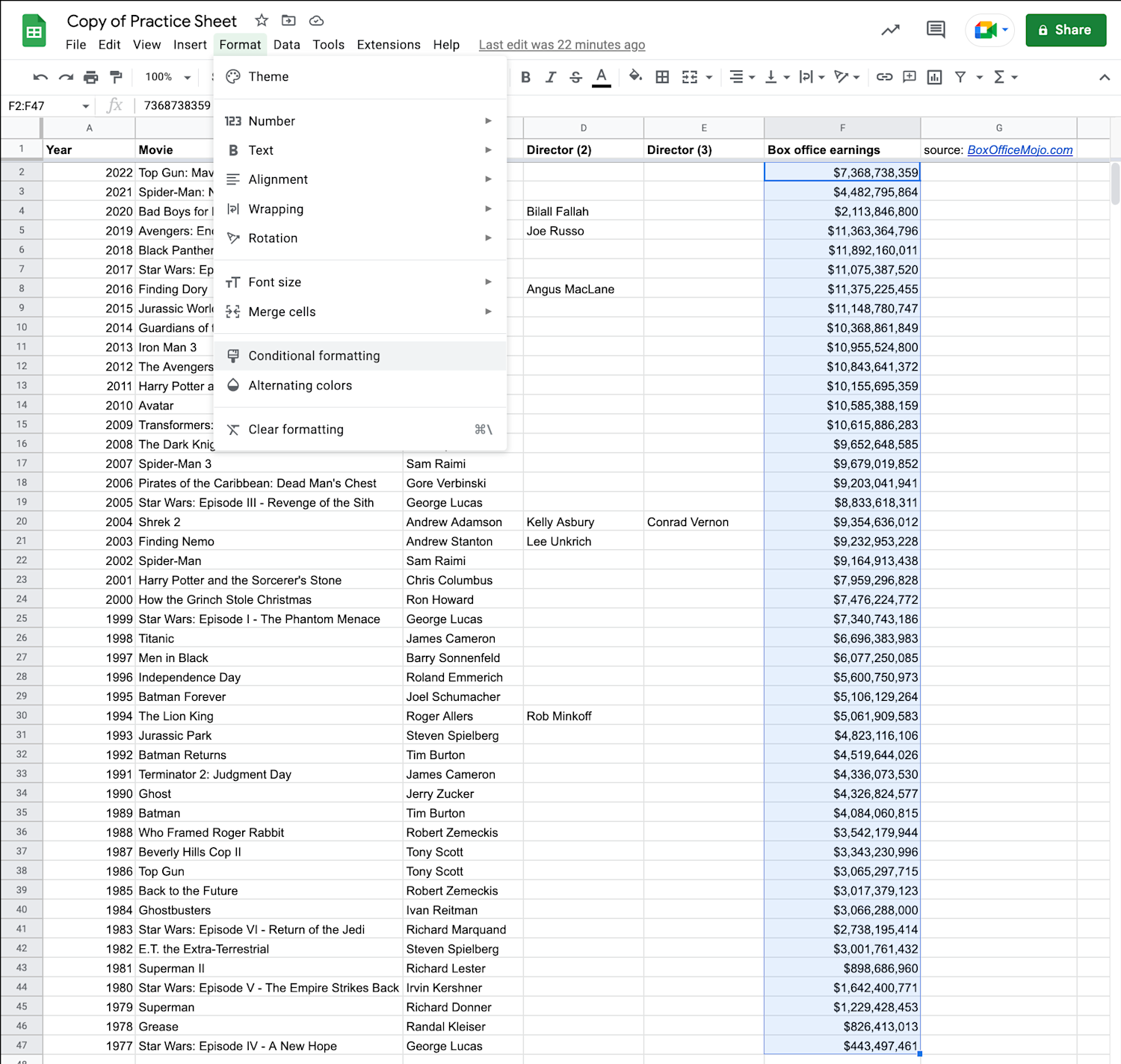
2. Click Format, then Conditional formatting.
Once you’ve selected your data range, click Format in the top menu. Then select Conditional formatting.
3. Select either Single color or Color scale.
Once you’ve clicked Conditional formatting, a menu will appear along the right side of the spreadsheet. You can select from two types of conditional formatting: Single color and Color scale. Pick the option that works for your needs:
Single color applies one color or format to cells that meet a specific condition, such as applying red to any cell containing a number below zero. You can also add multiple formatting rules to your data range, so that other colors are applied to cells in the same range that meet different conditions. For example, you can apply green to any cell containing a number above zero.
Color scale applies a color gradient to your data range, so that specific colors are associated with the maximum, minimum, and midpoint of your range. The numbers between these three values will be a gradient color. For example, you may apply a color scale that colors maximum values green, minimum values red, and the midpoint white, so you can identify financial figures that fall below or above expectations. In Color scale, you can apply multiple formatting rules to your range, but usually only one formatting rule is required, as all cells within the range will be colored by a gradient.
4. Apply color formatting in Google Sheets rules.
The formatting conditions for Single color and Color scale are slightly different from one another. Learn what you need to know about each one:
Single color formatting rules
Single color applies a single color to any cell that meets the condition specified by a rule.
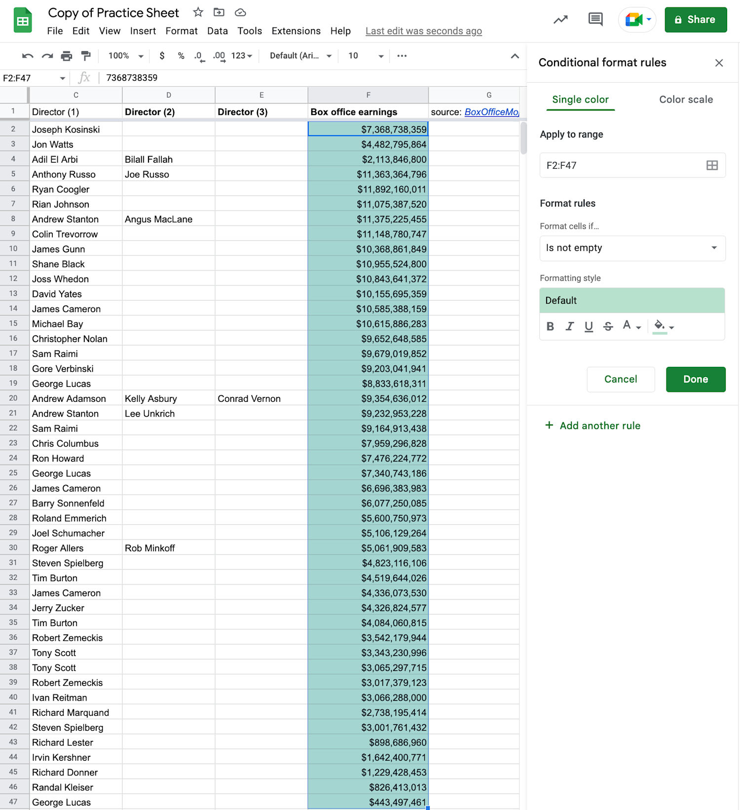
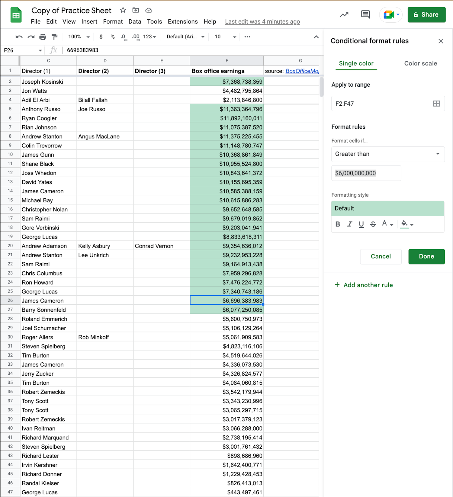
In Single color, you can specify the range to which you’d like the formatting rule applied, the rule itself, and the format for cells that meet the conditions set by the rule:
Apply to range allows you to specify the range to which you’ll apply the rule. If you didn’t select the range in the previous step, this is another way to do so.
The Format rules section contains a subsection called Format cells if…, which allows you to choose the condition that a cell must meet for the formatting to be applied. In total, you can apply nineteen rules to your data range.
The Formatting style subsection allows you to pick the format of the cell that meets the condition, including its color or whether you’d like it to be in bold, italics, underlined, or struck-through.
In the example below, the range selected is F2:F47, the selected rule indicates that formatting is only applied to cells containing a number greater than $6,000,000,000, and the formatting style is just the color green. This means the color green will appear on any cell within the range containing a number greater than $6,000,000,000.
Color scale formatting rules
Color scale will apply a color gradient to each of the cells contained within your range, as specified by the criteria for the applied rule.
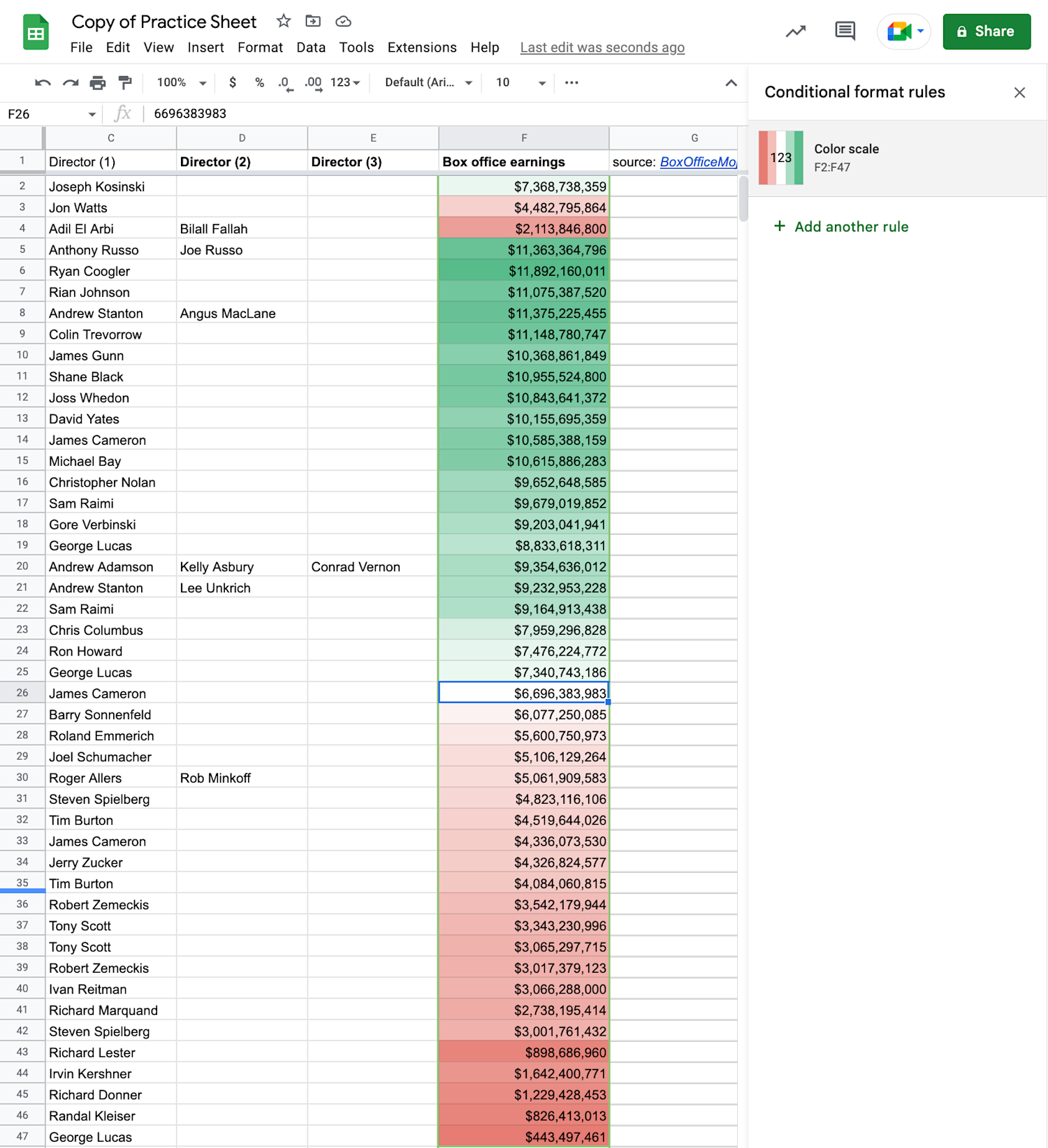
In the Color scale menu, you can control the range to which you’ll apply conditional formatting, the color gradient that will be applied to the range, the value types that will be formatted, and the minimum, maximum, and midpoint values that will be formatted:
Apply to range allows you to select a data range to which you will apply the conditional formatting rule.
Format rules is where you will select the specific rule you will apply to your data range. Select either a preset color scale or compose your own, and preview what the gradient will look like when applied to your range.
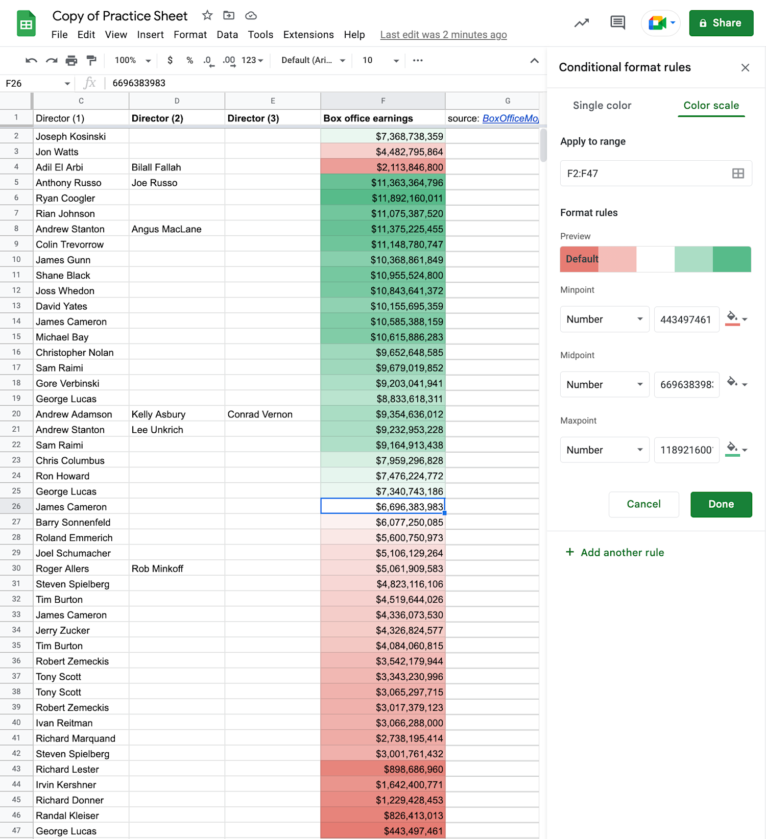
Below the preview, you’ll be able to set the minimum, middle, and maximum values to which you’ll be applying your formatting rule, as well as the color you’d like applied to each. These are called the Minpoint, Midpoint, and Maxpoint, and each can be set as either a value, number, percent, or percentile.
In the image below, the range selected is F2:F47, the preview shows a red to green gradient, and the minpoint, midpoint, and maxpoint have all been specified as numbers within the range. The lowest value will be red, the middle value will be white, and the maximum value will be green.
5. Click Done.
Once you’ve selected the rules and formatting you’d like applied to your data range, click Done. Conditional formatting will now be applied to the range you selected. If you would like to add another rule to your data range, select + Add another rule and repeat the process. If you’d like to delete the conditional formatting, click the trash bin beside the rule.
Conditional format rules: Google Sheets glossary
You can use 19 different rules within single-color conditional formatting. If you’re wondering which one to choose, consider what each one does:
Is empty: The cell contains nothing.
Is not empty: The cell contains something.
Text contains: The cell contains text with a specified element (e.g., text contains “sold”).
Text does not contain: The cell contains text without a specified element (e.g., text does not contain “sold”).
Text starts with: The cell contains text that starts with a specified element (e.g., text starts with “Tuesday”).
Text ends with: The cell contains text that ends with a specified element (e.g., text ends with “ready for processing”).
Text is exactly: The cell contains specific text (e.g., text is exactly “processing”).
Date is: The cell contains a specified date (e.g., 11/27/1992).
Date is before: The cell contains a date before a specified date (e.g., before 12/04/1991).
Date is after: The cell contains a date after a specified date (e.g., after 05/27/2016).
Greater than: The cell contains a value greater than a specified value (e.g., greater than 42).
Greater than or equal to: The cell contains a value greater than or equal to a specified value (e.g., greater than or equal to $123,456,789.00).
Less than: The cell contains a value less than a specified value (e.g., is less than 42).
Less than or equal to: The cell contains a value less than or equal to a specified value (e.g., is less than or equal to 42).
Is equal to: The cell contains a value that is exactly equal to a specified value (e.g., is equal to $123,456,789.00).
Is not equal to: The cell contains a value that is not equal to a specified value (e.g., is not equal to 42).
Is between: The cell contains a value between two other values (e.g., is between 1 and 100).
Is not between: The cell contains a value that is not between two specified values (e.g., is not between 30 and 70).
Custom formula is: This option allows you to input a custom formula that describes your rule.
Google Sheets conditional formatting based on another cell
Sometimes, you may want to format a range based on the value contained within a single cell, such as when you want to identify values within a column that are greater than, equal to, or less than a number contained within another cell. Take these steps:
Highlight your data range.
Click Format > Conditional formatting.
Select Single color.
Under Format rules, select Custom formula is as the applied rule.
Input your desired formula. Some formulas you might use, include:
Greater than or equal to a value in another cell: =$A1>=$B$1
Cell is not blank: =Not(ISBLANK([A1]))
Cell equals specific text: =A1="text"
*(Replace A1 with the first cell in your selected range, and adjust $B$1 or "text" as needed.)
Select the formatting style you’d like applied to the cells that meet the rule’s condition.
Click Done.
Conditional formatting duplicates Google Sheets
Learn how to highlight duplicates in Google Sheets using the steps above with a custom formula.
Troubleshooting Google Sheet conditional formatting
One common error when using conditional formatting is that your rule is not applying to all the cells you want it to.
To troubleshoot, check the range in Apply to range and make sure you have the cells you want formatted within it. The range must be separated by a colon, such as A1:A15. In this example, A1 is the first cell of column A, A15 is the fifteenth cell of column A, and the colon denotes that you are specifying a range between the two.
Learn more: How to Create Custom Error Bars in Google Sheets
Get more Google Sheets tutorials and career resources
Access additional Google Sheets tutorials on various topics, including pivot tables, freezing rows, and making a graph, and subscribe to Career Chat for up-to-date career advice. Take a look at these additional free resources:
Explore a data career: Career Paths in Data Analysis: Decision Tree
Watch on YouTube: Data Analytics Projects for Beginners: Where to Start
Sync your software: How to Sync Google Sheets with Google Calendar | Coursera
Whether you want to develop a new skill, get comfortable with an in-demand technology, or advance your abilities, keep growing with a Coursera Plus subscription. You’ll get access to over 10,000 flexible courses.

Coursera Staff
Editorial Team
Coursera’s editorial team is comprised of highly experienced professional editors, writers, and fact...
This content has been made available for informational purposes only. Learners are advised to conduct additional research to ensure that courses and other credentials pursued meet their personal, professional, and financial goals.