How to Use VLOOKUP in Google Sheets

In Google Sheets, VLOOKUP is a function that enables you to quickly find a piece of information in your spreadsheet that’s related to a known piece of information. The syntax for VLOOKUP is:

=VLOOKUP(search_key, range, index, [is_sorted])

You may use it to answer a specific question using your dataset. For example, if you have a spreadsheet with employee names and job titles, you can use VLOOKUP to answer questions like “What is Susie’s job title?” or “Who is the project manager?”

By the end of this tutorial, you will be able to use the VLOOKUP function to find a specific piece of information in your spreadsheet, and recognize when you might want to use an alternative function, such as HLOOKUP or XLOOKUP.

VLOOKUP formula

The VLOOKUP syntax is:

=VLOOKUP(search_key, range, index, [is_sorted])

Here’s a quick breakdown of the inputs:

• search_key: The known value that corresponds to the information you’re looking for

• range: The entire area on your spreadsheet to search within

• index: The number of the column your piece of information is in relative to the range

• Is_sorted:(Optional) For an exact match for your search key, write FALSE and for an approximate match for your search_key, write TRUE

How to use VLOOKUP

VLOOKUP stands for vertical lookup. You should use this function when your data is organized in columns, meaning each column lists a specific criteria, and data is related across each row.

If your data is organized in rows, with related data down each column, you’ll want to use HLOOKUP (horizontal lookup). We’ll discuss HLOOKUP later in this article. Here, we’ll detail, step-by-step, how to use VLOOKUP.

Ready to deepen your knowledge of Google Sheets?

To begin, you'll need your tab open to your spreadsheet. If you’re not already working with your own data set and want to follow along with our examples, make a copy of this template to practice. 

1. Decide where you want this information to appear.

You’ll type the VLOOKUP function into an empty cell on your spreadsheet, so your first step is to decide where you want your answer to appear.

With your data organized in columns, it’s typically a good idea to keep your VLOOKUP formula in a separate column to the side of your data rather than in a row above or below your data. This can make it a little easier to stay organized if you want to add new rows, sort, or filter your data. If you prefer, you can also create a separate sheet (tab) in your spreadsheet to house your functions.

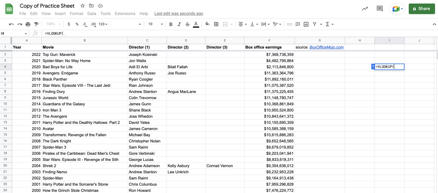
If you’re following along with the Practice Sheet, I’m going to start my VLOOKUP function in cell I4 by typing =VLOOKUP(.

2. Determine your search key.

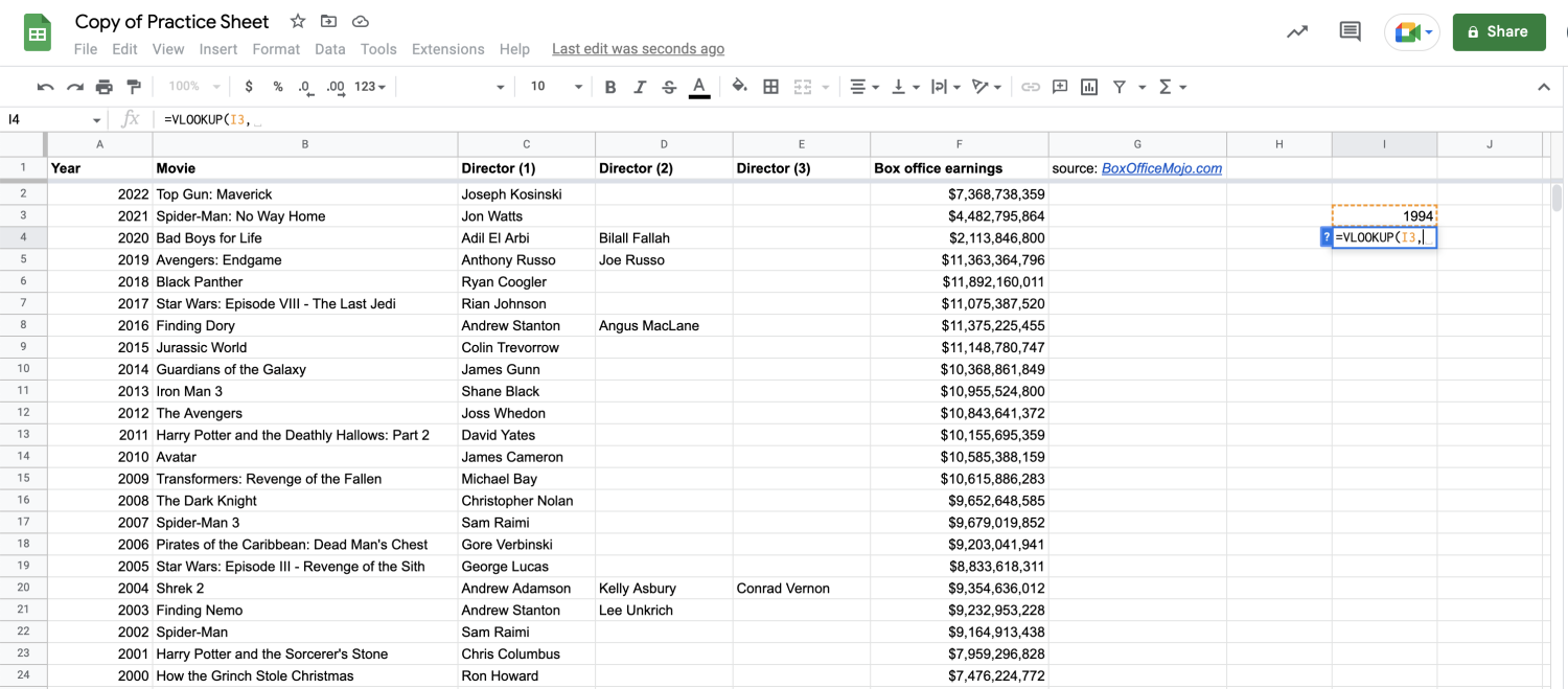
Your search key is the known value that corresponds to the information that you’re looking for. In our Practice Sheet, if you want to know what movie topped the box office in the year 1994, your search key would be 1994.

You can either type your search key directly into the function or you can reference a specific cell on your spreadsheet. Typing your search key into a new cell and referencing the cell in your function enables you to quickly answer multiple questions with your VLOOKUP function. Rather than retyping the function with multiple search keys, you can use the same function to find the movies that topped the box office in 1994, 1995, and 1996 by simply changing the text in your referenced cell.

In my Practice Sheet, I’m going to reference cell I3 for my search key, and in cell I3 I’ll write 1994. Now, my function reads =VLOOKUP(I3,.

3. Identify your range.

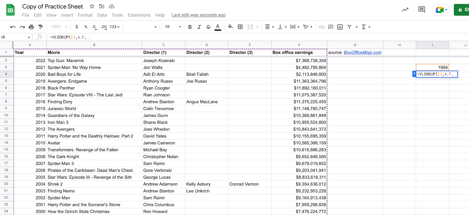
Your range is the entire area on your spreadsheet to search within. If you highlight the entire area where your data is, the range would be denoted [top left cell]:[bottom right cell]. If your range includes entire columns, you can denote your range [leftmost column]:[rightmost column].

When using VLOOKUP, your search key should be found in the first column of your range, and the related information you are seeking should be found in a column to the right of that column. This is one limitation of the VLOOKUP function—it can only search left to right. If your search key is in a column to the right of the information you’re seeking, you’ll need to use the XLOOKUP function. We’ll go into more detail about XLOOKUP below.

In my Practice Sheet, I’ll write my range as A:F. I could also write my range as the more exact A2:F47, but then I’d have to remember to adjust my VLOOKUP function if I ever add new rows of data pertaining to future box office-winners. Now, my function reads =VLOOKUP(I3,A:F,.

4. Count columns in your range to find your index.

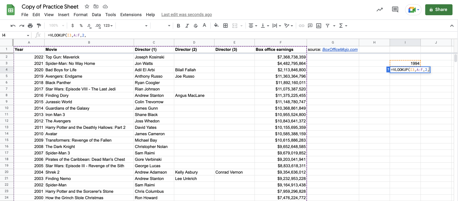
Your index is the number of the column your piece of information is in relative to the range. This will always be a positive integer.

To find your index, start with your first column as 1 and count over to the column where your range will be found.

In my Practice Sheet, I am looking for a movie title, which I know is found in column B, or the second column within my range, A:F. My index is 2, so now, my function reads =VLOOKUP(I3,A:F,2,.

5. Answer is_sorted with TRUE or FALSE.

For the final input, you’ll either write TRUE or FALSE. If you want an exact match for your search key, write FALSE; if you want an approximate match, write TRUE. This input is optional and will default to TRUE if you don’t use it, but generally, FALSE is considered the best practice here.

In my Practice Sheet, because I want an exact match, I’ll write FALSE, then close out our function with a parenthesis: =VLOOKUP(I3,A:F,2,FALSE).

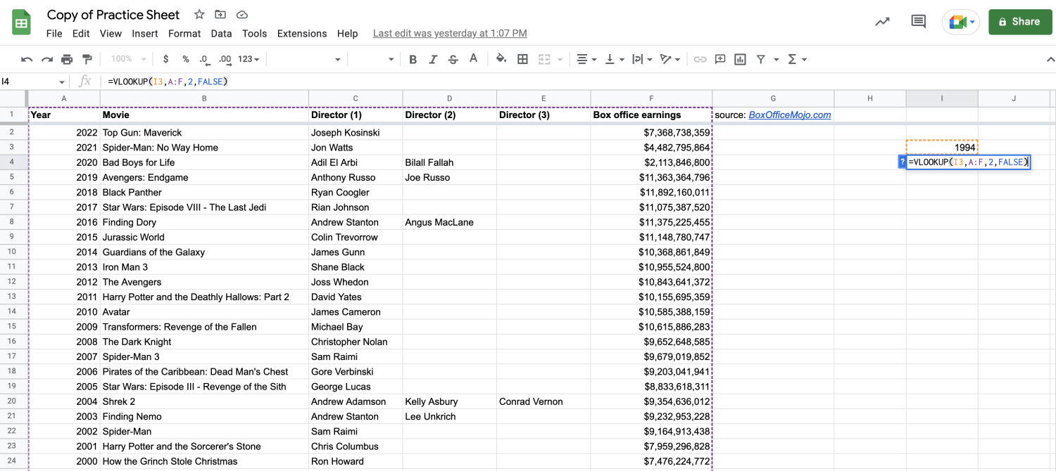
Hitting Enter on my keyboard will reveal the answer to our question: the highest-grossing movie of 1994 was Disney’s instant classic, The Lion King!

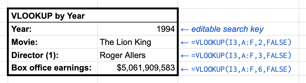
Optional bonus step: Formatting your VLOOKUP for repeat use

If you plan to use your VLOOKUP function to answer multiple questions, it may be helpful to add labels and formatting around your function. You can also add additional VLOOKUP functions to quickly pull even more data related to your search key.

For example, in my Practice Sheet, I supplemented the movie title VLOOKUP function with additional functions to pull the primary director and box office earnings, all tied to the original search key in I3. I also added labels in the column to the left of my functions so that I can clearly see what data my VLOOKUP functions will pull, titled my functions in the row above my search key to easily recall my question, and added borders to differentiate my functions from the rest of the data on my sheet.

Now, I am able to quickly answer several questions about the highest-grossing movie in any given year by simply changing the year named in cell I3.

Related VLOOKUP tasks

Here are some more ways you can use VLOOKUP in Google Sheets:

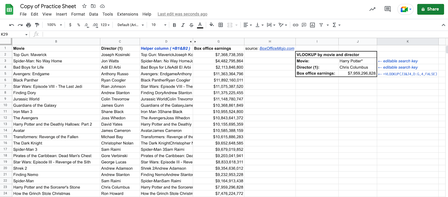
VLOOKUP with multiple criteria

You can only use one search key in a VLOOKUP function, but there are workarounds if you want to look up some information with two (or more) search keys. The most common way to approach a VLOOKUP with multiple criteria is to create a “helper column.”

A helper column is essentially an additional column that you create that joins your two pieces of criteria into a single column. You can do this using a formula, =[cell]&[cell].

Then, in your VLOOKUP function, your search key joins your two pieces of criteria in a similar manner. If you’re referencing cells in your workspace, you can format your search key as [cell]&[cell], or you can type out the information you’re looking for directly into the function, [criteria1]&[criteria2].

Take a look at the image below to see how to use a helper column and two search key cells to find out how much money the Harry Potter movie directed by Chris Columbus made.

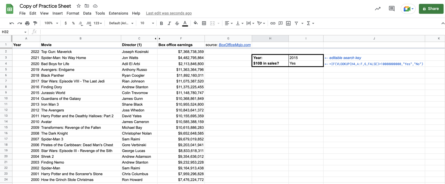
VLOOKUP with IF statements

If you’d like to answer a yes or no question using your data, you can wrap an IF function around your VLOOKUP function. This will return custom text under specific conditions.

To do this, you use a regular IF function, = IF(logical_expression, value_if_true, value_if_false), with your VLOOKUP function as part of your logical expression.

Take a look at the image below to see how to use an IF function to answer whether the top box office earner in a given year earned more than $10 billion in sales.

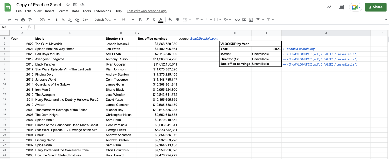
VLOOKUP with IFNA statements

You can use your VLOOKUP with an IFNA function to return custom text if your search key can’t be found. Your custom text will show up instead of a #N/A error.

To do this, surround your VLOOKUP function with an IFNA function:

=IFNA(VLOOKUP(search_key, range, index, [is_sorted]),“[return_value]”)

Take a look at the image below to see how to use an IFNA function to return the phrase “Unavailable” if you try to find box office data for a year outside of the data set, 1977-2022.

Common VLOOKUP errors and solutions

If you don’t write your function accurately, you’ll get a formula parse error. Here are some common error messages associated with VLOOKUP and some suggestions for what you can do to troubleshoot:

• #NAME?: A name error indicates that one of your inputs is unexpected. For example, if you write a letter instead of a number for the index, or if you write NO instead of FALSE for is_sorted. Google Sheets functions follow certain language conventions, and this error tends to show up if an input falls outside of those conventions.

• #REF: This error indicates that your index is outside of your range. When you are counting your index, make sure you are only counting the columns within your identified range starting with one for the first column. For example, if your range is columns B through D (B:D), B would be index 1, C would be 2, and D would be 3. Using an index 4 here would return a #REF error.

• #VALUE!: This error usually indicates a problem with your index, such as using a negative number or zero. Make sure you are using only positive integers as your index, counting the columns within your range from left to right, with your search key found in the first column in your range.

• #N/A: This error indicates that your search key can’t be found within your first column. Check that you’ve spelled your search key correctly and used correct punctuation throughout your function.

• Returns the wrong value: There are a few common reasons a VLOOKUP function will return an incorrect value:

  • This could be related to the is_sorted input. If you leave that input blank (so default to TRUE) or write TRUE, but your first column isn’t sorted in ascending order, you’ll return an incorrect value. Try sorting your column or changing is_sorted to FALSE.

  • This could be related to the data set. If your search key shows up multiple times in your first column, VLOOKUP will only return the value associated with the first mention of your search key.

  • This could be related to your data cleaning process. VLOOKUP is not case sensitive, but it is sensitive to extra spaces and characters. Make sure you’re working with clean data and using the same character conventions in your data set and search key.

Read more: How to Fix Formula Parse Error: Google Sheets

Limitations and alternatives

VLOOKUP is a vertical lookup, meaning it searches columns, and it only searches from left to right. If your data is organized differently, you may want to use a different, but similar, function to perform your lookup.

VLOOKUP vs. HLOOKUP

HLOOKUP is a horizontal lookup. Use an HLOOKUP function if your data is organized by rows.

The syntax for HLOOKUP is:

=HLOOKUP(search_key, range, index, [is_sorted])

You’ll notice that the syntax for HLOOKUP is almost identical to that for VLOOKUP. The difference is you consider rows instead of columns. Your search key should be found in the first row of your range, and to find your index, you should count rows instead of columns.

VLOOKUP vs. XLOOKUP

XLOOKUP is a newer function in Google Sheets which enables you to look up data in any direction.

The syntax for XLOOKUP is:

=XLOOKUP(search_key, lookup_range, result_range, missing_value, match_mode, search_mode)

This syntax looks more complex than VLOOKUP, but several inputs are optional. In its simplest form, you only need to type =XLOOKUP(search_key, lookup_range, result range).

Here’s a quick breakdown:

• search_key: Similar to VLOOKUP, this is the known value that corresponds to the information you’re looking for

• lookup_range: The singular column or row on your spreadsheet where your search key will be found

• result_range: The singular column or row on your spreadsheet where your result will be found

• missing_value: (Optional) The custom text you’d like returned if your search key can’t be found. If left blank, this will default to #N/A.

• match_mode: (Optional) How you’d like to search the lookup_range for the search_key, either:

  • 0 for an exact match (default, if left blank)

  • -1 for an exact match or, if unavailable, a match less than the search key

  • 1 for an exact match or, if unavailable, a match greater than the search key

  • 2 for a wildcard match

• search_mode: (Optional) How you’d like to search the result_range, either:

  • 1 to search from first entry to last (default, if left blank)

  • -1 to search from last entry to first

  • 2 to search with binary search with the range sorted in ascending order

  • -2 to search with binary search with the range sorted in descending order

Keep learning

Interested in strengthening your abilities to work with data using Google Sheets? Enroll in the Google Data Analytics Professional Certificate. You’ll learn more about spreadsheets and other key analysis tools.