How to Use Google Sheets MATCH
Read this article to learn what the Google Sheets MATCH function is and how to use it, how to troubleshoot it, and how it differs from VLOOKUP.
![[Featured Image] A person uses Google Sheets MATCH on their office computer.](https://d3njjcbhbojbot.cloudfront.net/api/utilities/v1/imageproxy/https://images.ctfassets.net/wp1lcwdav1p1/3K7FnbMdu6gvddmPLNGW1d/a752f72f72cdb5f2d400f31fe5eb51a1/GettyImages-1353281811.jpg?w=1500&h=680&q=60&fit=fill&f=faces&fm=jpg&fl=progressive&auto=format%2Ccompress&dpr=1&w=1000)
Key takeaways
The Google Sheets MATCH function finds a specific item you want to look up and tells you the position of that item in the range.
The MATCH function allows you to create your own search engine of sorts to find the relative position of cells containing a specified value (either numbers, text, or dates) in the selected range of cells.
To use Google Sheets MATCH, select the cells in one row or column that you want to search, access the MATCH function through the Insert menu, and add your parameters using the built-in syntax.
You can also use the VLOOKUP function to conduct a more robust search that can extend beyond the cells in a single row or column.
Use this tutorial to learn how to use the MATCH function, with steps you can try at your own pace. Then, if you're ready to learn more about how to analyze data with Sheets and beyond, consider enrolling in the Google Data Analytics Professional Certificate, where you can learn in-demand skills and get AI training from Google experts.
How to use the Google Sheets MATCH function to find matching cells
Follow these three steps to use the MATCH function:
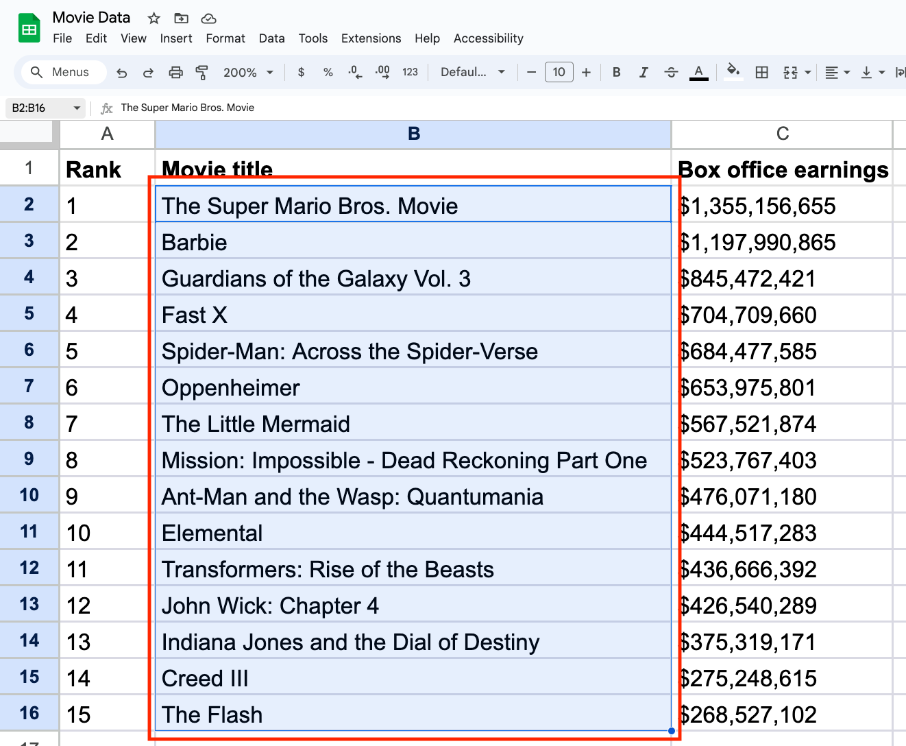
1. Select a cell range in Google Sheets.
Open Google Sheets in your web browser and select the cells you want to include in your match. When selecting your range, consider that the MATCH function only allows a range of one single row or column, not multiple or mixed. Selecting multiple rows or columns as your range will prompt an error.
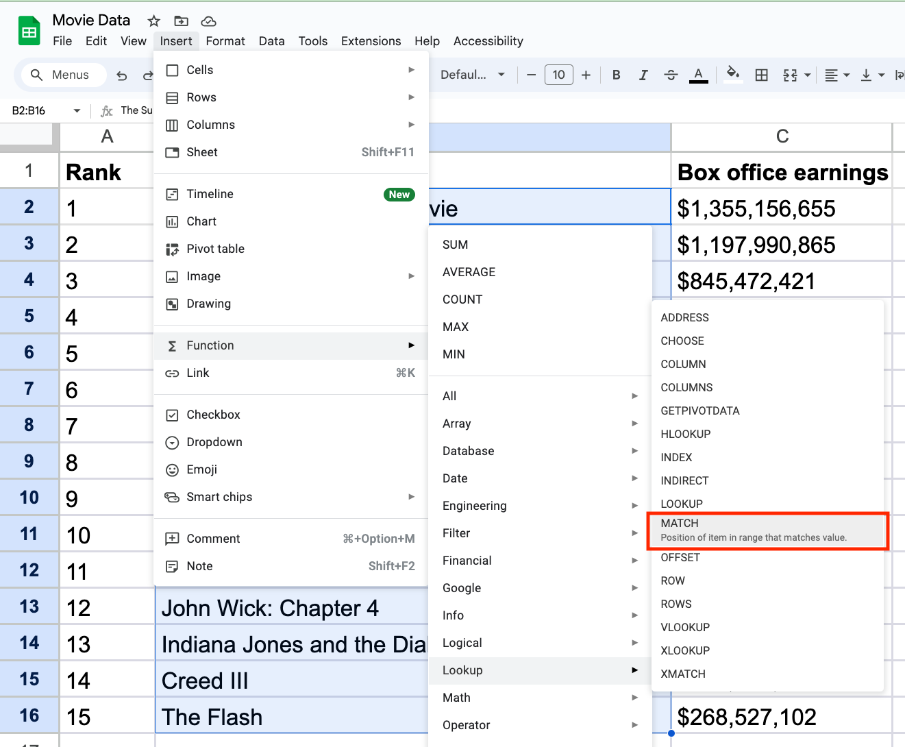
2. Use the MATCH function to locate the item within your cell range.
To choose the range that contains what you’re looking for, go to the toolbar menu and select Insert > Function > Lookup > MATCH.
As a shortcut, you can select an empty cell in your row or column and type =match( ).
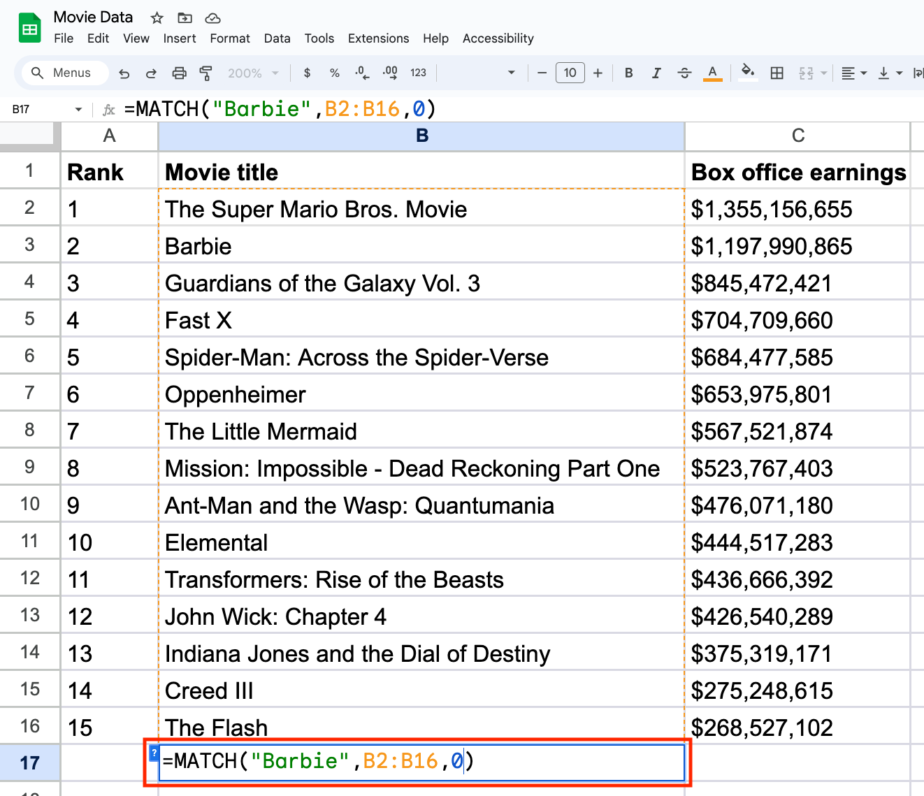
3. Enter the MATCH function parameters for your search.
The Google Sheets MATCH function has a built-in syntax that calls for three parameters: a search key, a range, and the search type.
=MATCH(search_key, range, [search_type])
search_key: Enter the numeric or text value you want to search for in your cell range. Use quotation marks (“ ”) around this parameter if it’s a text value (“apple”); this isn’t necessary for numerical values.
If you want to search for a date, use the “DATE (year, month, day)” format in the search key. For example, =MATCH( DATE (2023,12,31),...”
range: Enter the cell range (within a single column or row) where you want to search for the value—the start and end of the range will be separated by a colon (:).
search_type: This parameter specifies how the function should perform the match. You can enter a 0 to find an exact match, 1 for an approximate match less than or equal to the search_key (when range is in ascending order), or -1 for an approximate match greater than or equal to the search_key (when range is in descending order). If you don’t enter a search type, it will default to 1.

For example, if you want to find the exact match of the word “Barbie” anywhere between B2 and B16, your function would read as follows: =MATCH("Barbie", B2:B16, 0)
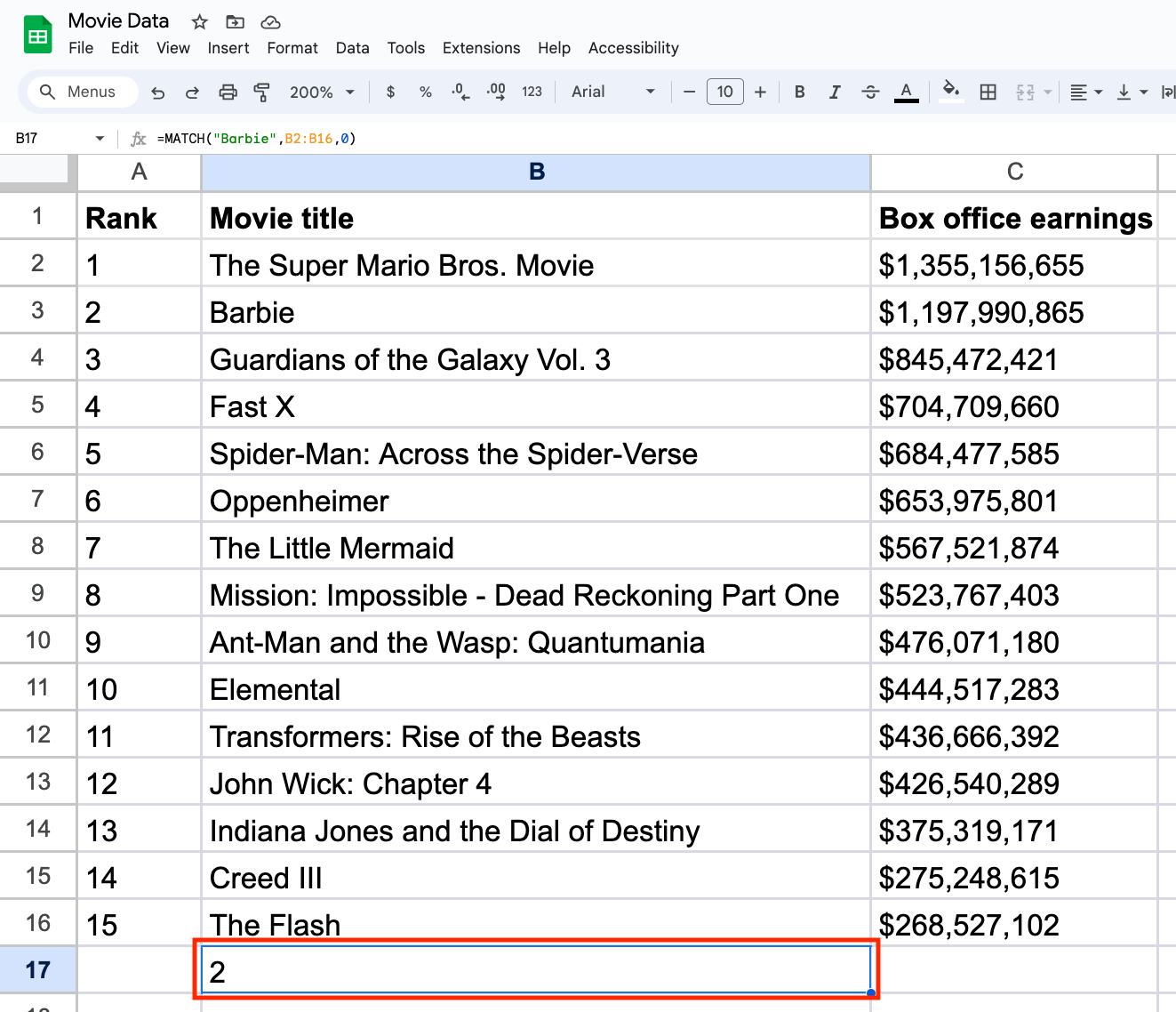
Once you fill out these parameters, press the Enter key on your keyboard to get your result. The function will return a number representing the position of your value relative to the beginning of the specified cell range. In our example, “Barbie” is located in the second position in the cell range we entered.
How to troubleshoot the Google Sheet MATCH function
You might encounter an error when using the Google Sheets MATCH function for several reasons. If you’re sure the data is in the spreadsheet but can’t locate it when using the MATCH function, check the cell for any unexpected characters. Even a minor typo could produce an error.
Other things that can lead to an error include:
Not typing in the exact search term you’re looking for
Leaving the range blank
Adding an incorrect search type
Choosing the wrong range
Learn more: REGEXMATCH Google Sheets: A Beginner’s Guide
What is the difference between VLOOKUP and MATCH in Google Sheets?
The main difference between the functions MATCH and VLOOKUP is what they return and how they handle columns. MATCH will provide the position of the specified value in only a single row or column. However, VLOOKUP provides the coordinating value to your search term across another row or column. In our example above, MATCH returns “2,” the exact position of the word “Barbie” in the specified column. With VLOOKUP, you can find the exact box office earnings for the search key “Barbie.” VLOOKUP will search the first column of a given range and return the value of a specified cell in the row found.
Both functions have their advantages, but the choice between them should be guided by the specific information you need and the execution speed you require.
Explore more Google Sheets tutorials and free resources
Expand your expertise with Google Sheets functions with more free tutorials, including how to add numbers across a range of cells using the SUMIF function and using the =IMPORTRANGE to easily reference updated data from multiple sheets. You can also subscribe to our Career Chat newsletter to stay current on trends in your field. Take a look at these additional resources as well:
Watch on YouTube: 3 Essential Tools You’ll Learn in the Google Data Analytics Professional Certificate
Learn key terms: Data Analysis Terms & Definitions
Explore career paths: Career Paths in Data Analysis: Decision Tree
Whether you want to develop a new skill, get comfortable with an in-demand technology, or advance your abilities, keep growing with a Coursera Plus subscription. You’ll get access to over 10,000 flexible courses.

Coursera Staff
Editorial Team
Coursera’s editorial team is comprised of highly experienced professional editors, writers, and fact...
This content has been made available for informational purposes only. Learners are advised to conduct additional research to ensure that courses and other credentials pursued meet their personal, professional, and financial goals.