Dijkstra's Algorithm: Definition, How It Works, and Examples

Key takeaways

• Dijkstra’s algorithm is a greedy shortest-path algorithm that finds the most efficient route between a starting node and all other nodes in a weighted graph.

• Dijkstra’s algorithm time complexity depends on the graph's size and implementation, typically running in O(V lg V) for the main loop and O(E lg V) overall with a priority queue.

• Dijkstra’s algorithm examples in the real world include online maps and internet routing.

Developers can implement Dijkstra’s algorithm in Python to build tools like navigation systems and network routers. Learn more about Dijkstra’s algorithm and how it works to solve shortest-path problems.

If you’re ready to take your first step toward a career in computer programming, consider enrolling in the Meta Back-End Developer Professional Certificate to work with programming systems including Python syntax, Linux commands, Git, structured query language (SQL), and version control.

What is Dijkstra's algorithm?

Dijkstra’s algorithm calculates the lowest-cost route between a starting node and every other reachable node in a weighted graph with nonnegative edge weights. You can represent many networks today as weighted graphs, where edges connect nodes and carry numerical weights. The weights denote the “cost of travel” between the nodes. Dijkstra’s algorithm works when all weights are nonnegative. Dijkstra’s algorithm is a greedy algorithm; at each iteration, it moves to whichever unvisited node currently has the shortest distance from the source. For graphs with nonnegative edge weights, those local choices still produce the shortest paths.

Its name comes from Edsger Wybe Dijkstra, a Dutch computer scientist who introduced the algorithm in 1959.

What does Dijkstra's algorithm do?

Dijkstra’s algorithm is effective for finding the shortest possible path in a weighted graph, provided you know the weights associated with the edges. Shortest-path problems show up all around you. Without an efficient algorithm like Dijkstra's, finding the best route becomes increasingly expensive as networks grow.

Starting from the source node with a distance of zero, the algorithm calculates the shortest known distance to neighboring nodes. It picks whichever unvisited node has the smallest tentative distance, then checks its neighbors and updates their distances when a faster path opens up. The process continues until it has determined the shortest paths to all reachable nodes or reaches the destination node. It’s worth noting that negative weights can cause the algorithm to produce inaccurate results because it assumes all edge weights are nonnegative.

What is Dijkstra's algorithm used for?

Dijkstra’s algorithm is a popular tool used for pathfinding, network optimization, and routing because it efficiently finds the lowest-cost path even on large networks.

It’s part of applications that require the shortest path possible, like Google Maps. When you enter two addresses, Google Maps uses shortest-path algorithms to identify an efficient route between those locations within seconds. It is also helpful in internet routing, including the Open Shortest Path First (OSPF) protocol.

How does Dijkstra's algorithm work?

Dijkstra’s algorithm works by following four steps to identify the shortest possible path between nodes.

1. Start at the source node with a distance of zero.

2. Select the node with the shortest distance from the source.

3. Calculate the tentative distances for every adjacent node.

4. Repeat until you've processed all reachable nodes or reach the destination.

For example, imagine a small delivery network with four stops (nodes): A, B, C, and D:

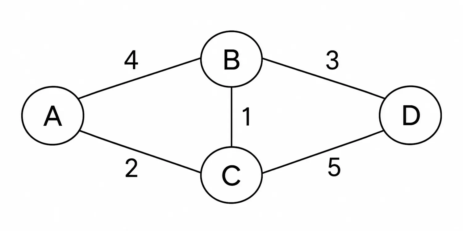
From A, you can reach B in four minutes or C in two minutes. From C, you can reach B in one minute or D in five minutes. From B, you can reach D in three minutes.

To find the shortest path from A to D, Dijkstra's algorithm starts at A and checks both neighbors (B and C). Then it moves to the closest one (C, in two minutes).

From C, it updates the distance to B, three minutes (2 + 1 = 3). This is shorter than going directly from A to B (4). It checks the distance to D: seven minutes (2 + 5 = 7).

Then it moves to B and checks B's neighbor D: six minutes (3 + 3 = 6).

After determining the shortest route, the algorithm returns the shortest path: A → C → B → D, with a total travel time of six minutes.

What is the time complexity of Dijkstra's algorithm?'

Dijkstra’s algorithm's time complexity varies based on the size of the graph and the implementation you choose. In one implementation of Dijkstra's algorithm, using a heap-based priority queue, the main loop runs in O(V lg V), where V represents vertices. Including the time spent processing edges, the total runtime comes to O(E lg V) for a connected graph. As the input grows, so does the number of steps the algorithm needs, which is what time complexity measures. The lower the time complexity, the more efficiently the algorithm runs. This is important when you’re running time-sensitive applications and need quick results.

Why a priority queue?

Many implementations of Dijkstra’s algorithm use a priority queue, a data structure that removes elements in priority order. This allows the algorithm to quickly select the unvisited node with the smallest known distance instead of repeatedly searching every unvisited node, improving efficiency on large graphs.

Read more: AI vs. Algorithm: What’s the Difference?

Dijkstra's algorithm example

For example, consider you need to map out the shortest route to the airport from your home. You open Google Maps and input both addresses. These become your source and destination nodes. Google Maps then uses shortest-path algorithms like Dijkstra’s to identify an efficient route between these two locations by comparing travel times and selecting the route with the lowest estimated travel time.

To implement Dijkstra’s algorithm, you will complete three stages: initialization, iteration, and termination.

1. Initialization

First, assign a source node (s) a tentative distance value of 0 (dist [s] = 0). Assign all other nodes a tentative distance of infinity (∞).

You can also initialize a predecessor map to reconstruct the shortest paths.

All nodes at this step are unvisited.

2. Iteration

Now, you select the unvisited node u with the smallest tentative distance.

Mark u as visited. Since edge weights can't be negative, no other path to u can turn out to be shorter, so its distance is now final.

For each neighboring v of u: calculate the alternative distance

alt = dist[u] + w (u,v)

If alt < dist[v], update dist[v] = alt and set predecessor[v] = u.

3. Termination

Once the algorithm has visited all reachable nodes or reaches the destination you're looking for, it terminates.

What are the limitations of Dijkstra's algorithm?

One of Dijkstra’s algorithm’s main limitations is its inability to work with negative edge weights. Negative edge weights can reveal a shorter path after Dijkstra's algorithm finalizes a node. Another potential drawback of Dijkstra’s algorithm is memory overhead, which can increase significantly as the size of the graph grows.

How do you implement Dijkstra's algorithm in Python?

Dijkstra’s algorithm is a practical choice when building real-world applications in Python, especially for developers working with networks and graphs. You can use Dijkstra’s algorithm to find the shortest path between nodes as a computer programmer while designing game AI, optimizing network routing, or creating a GPS navigation system.

When choosing a library to use for working with Dijkstra’s algorithm in Python, look for a library that fits your application. For example, a library that has the functionality required for mapping the shortest path between two points would be the right choice for a navigation system. It’s important to remember that existing code often serves as a starting point, and you’ll need to tailor it to your application. You can find MIT-licensed project source code on GitHub.

Build computer programming skills on Coursera

Subscribe to our Career Chat newsletter on LinkedIn for industry insights, career tips, and skill-building resources. Then, further explore different computer programming skills with our free resources:

• Watch on YouTube: How Long Does It Really Take to Learn Python?

• Read our Career Chat issue: 3 Machine Learning Projects to Build Your Skills and Portfolio

• Prepare for an interview: The Ultimate Python Interview Prep Guide

Accelerate your career growth with a Coursera Plus subscription. When you enroll in the monthly or annual option, you’ll gain access to over 10,000 courses.

Build job-ready skills with Coursera Plus

Start 7-day free trial

• 
• 
• 
• 

Start 7-day free trial