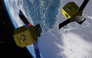
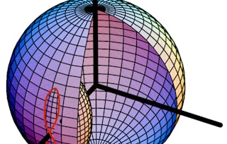
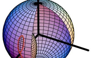
0:20
And you have some quadratic parts in there, not too bad, over 4.
 So this B matrix, we typically pull out the scalar in my book, so
 you will see it's this B matrix over 4.
 So when you linearize, this B matrix basically vanishes to identity, and
 you get again MRP rates relate to omega as simply being omega over 4.
 So this'll be important when we do feedback control, and linearize,
 and so forth.
 So that's why the 1/4 is outside of the B matrix.
 So in your mind, you remember, angles over 4.
 But this is a convenient form, it's very nice to program.
 You've got a scalar times identity operator.
 You could cross product operator and vector out of product operator.
 So when you have to do algebra, I'll show you one of them.
 Don't do it in the matrix component form again really look to use this formula.
 And you can do these properties, derivations and proofs very,
 very quickly, very, very compactly.
 2:05
Orthogonal right, which is very nice so it's easy to invert and
 bring it over that's why this buffered form was convenient.
 If just integrating MRPs you don't need this first column because this first
 column times 0 is always going to vanish.
 So you typically see a four by three version of this but
 if you have to do an analysis, this buffered form is very, very convenient.
 So a nice property people go well, quaternions, differential kinematic
 equations, that B matrix can be orthogonal, that's beautiful, very handy.
 Well, let's see what MRPs do.
 2:37
So, with the MRPs,
 if you have to invert it while you can always invert the matrix booth force.
 And there was a fact there were 4 that comes over, so
 it's 4 times B inverse times the MRP rates.
 Now, this matrix is not orthogonal but
 it's called near-orthogonal by this definition.
 The inverse of a B if it were equal to B transpose it would be orthogonal.
 But here it's equal to B transpose times a scalar, that's it.
 3:10
So, it's almost orthogonal,
 you just have that one scalar parameter you have to account for.
 And if you're doing analysis,
 especially there was some papers we wrote on perfectly linear, closely dynamics.
 Another thing is where we have to do these things analytically.
 And you have to take B inverse everywhere, only happen to do with transpose times
 the scalar, saves you weeks of life of having to this stuff.
 So, it's a very convenient formula.
 You end up having to prove this,
 this is something I'd expect you to be able to do it in the exam.
 3:40
So the way you prove this property is you look at B times B transpose.
 If this was orthogonal, this would give you identity matrix, right?
 But if you just carry out the math of B times B transpose,
 you will get identity matrix times a scalar, right?
 And so, if you bring the scalar over and matrix times something giving you identity
 that's something has to be matrix inverse, that's the only way
 matrix can something gives you identity at least for general matrices.
 And that's how you could then argue that something has to be the inverse so
 therefore it's a transpose times scalar.
 But to do this B times B transpose, don't use this, use this definition.
 because when you need to carry out there's chain rules,
 you have identity times identity.
 You will have identity times tilde, identity times this.
 You will have sigma tilde times sigma sigma transpose.
 What's going to happen with those products?
 Sigma tilde times sigma sigma transpose.
 Tony, what do you think?
 Do we have to carry this math out?
 Sigma tilde times sigma sigma transpose.
 4:51
>> Zero.
 >> Zero, right?
 because sigma tilde sigma is basically sigma cross with sigma.
 Whatever else you do with that math it's zero times something it's all going to be
 zero in this case in simplistic terms, right?
 But you can see this is without doing all this stuff and
 things have to cancel, you can do it in this form, carry out the components, and
 you will quickly end up with something that gives you the answer.
 So that's how you should solve that kind of a problem and
 you'll be done in a fraction of the time.
 5:31
Talked about integrators just a little bit earlier.
 I'm just going to get a new fresh page.
 So we have, sigma dot = 1/4,
 this B matrix times omega it's basically what you have.
 We've done a problem where you have to integrate Euler angles basically of
 this form.
 You assume for now that omega is something known, right, that's back there.
 6:26
And in that time loop let's do a 4, 5.
 Easy, well then, you have to compute the k1 term,
 k2, k3, k4, right?
 And if this is in state vector form, x = sigma,
 x dot = f(x) which in this case is just
 1/4 B omega, well, omega matrix.
 So that's your equation that you're that you're solving,
 you call this thing 4 times with different inputs, right?
 And then at the end the new state, you would say, okay, so
 we say, x = sigma naught.
 But then I say, xn+1 = xn + all these k's are in here,
 they get blended together, right?
 And that gives you your step and you're done.
 7:57
>> At each time step you have to check, the denominator is close to zero?
 >> You don't check the denominator, that's the addition part you are thinking.
 >> Okay.
 >> How do we know we have to switch MRPs?
 How do we know an MRP describes a 180 degree or more rotation, [INAUDIBLE]?
 >> Back it's magnitude?
 >> It has to be what value?
 >> Above 1.
 >> 1, right?
 So for MRPs, think of the one surface.
 It's what describes something being completely upside down,
 that's it about any access, right?
 So we are checking for the norm of MRPs being greater than 1,
 that means I'm describing a.
 Do you do that here?
 Do you do it inside of this f function?
 8:54
>> Do you want to do it here?
 >> [INAUDIBLE] >> Or here?
 >> Can you do it up above before you [INAUDIBLE], Yeah.
 >> Your voice is fading off, I can't hear a thing.
 >> [LAUGH] I think, I'm trying to think of how you will do it,
 but if you can do it before you feed the inputs into the integrator then you could
 keep your integrator stand [INAUDIBLE], >> Okay.
 >> Problems.
 >> Okay, so you're saying here, basically.
 This is the integrator part.
 Let me just circle that with color.
 9:47
>> Average.
 >> You could, right?
 If your input is 190 degrees.
 And hope infinity because there's a 360.
 Otherwise you're just being cruel, you go smack him a few times, okay?
 But assuming it's finite, you could check here if you wanted to and
 say, upfront, am I close to 180?
 If yes, I simply switch that.
 10:17
Same thing with the quaternions.
 We had one set of quaternion, beta naught equal to this 4x3 matrix times omega.
 It didn't matter if it's a long or
 short rotation, they had the same differential kinematic equation.
 The same thing holds here.
 So we don't have to switch our equations that we're integrating.
 I just have to switch, hey, I'm not at 190, I'm actually at minus 170.
 And then, the same math holds.
 So, you could do that here, that would work or
 very often I assume this is a good input.
 I do it at the end of the integration steps.
 So, if I feed it back to the other routines, different things,
 I tend to put it right here.
 And this is as if I'm checking if the norm of sigma > 1,
 then I'm simply saying sigma ends up being minus sigma/sigma squared
 has basically, whatever sigma measure you're having your code,
 I'm reversing the sign and dividing by the norm squared.
 11:16
because I'm not counting on being precisely on 1.
 So if you have really time step, you're tumbling quickly,
 you may have jumped 285 degrees, quite a bit past 180, no problem.
 Nothing bad happens at 180, it's purely a choice to switch there.
 In fact, there's some papers who talk about switching at general surfaces
 another kind of stuff,
 but there's no practical benefits that I've seen, it's just nice mathematics.
 11:58
David.
 >> Daniel.
 >> Daniel, Bobby, this is not my day for names.
 >> You might get different k's, one of the functions might decide to flip, it might,
 and the other won't.
 >> Yeah, so what can happen is you're right around 180, right?
 And with this you're doing some at the current time step, the rates,
 then half a time step forward, then a full time step forward.
 And you're blending them, and in that time step you might be switching through 180.
 And then so some answers are around 180, the other answers
 are around minus 180, and I blend them together and I get 0.
 And that's not more precise, it's plain wrong, okay?
 So here, just one of the things, people always to this,
 I'm just going to highlight it again.
 That switching has to happen outside.
 So, Trevor, you had a good idea.
 You don't want to do it inside the integrator block.
 Let it do it's thing, we're not operating around, bad things happen.
 Nothing, just let it do it's thing, and
 just make sure you put it in a sensible place.
 You could put it up top, I tend to put it on the bottom, either works, right?
 That's where you want to do the switching, and
 then you just keep in chugging along, that's it.
 So with that one little if statement, I can do with the three parameter set,
 I'm not introducing quarternian constraints.
 Otherwise, my attitude control problem of something tumbling freely in space becomes
 immediately a constrained integration problem, is in fact with the quaternions
 after you've integrated, you probably have to go and renormalize your quaternions.
 because with integration errors they don't stay at unit norm, they become 1.000001 or
 something, right?
 And if checked, it would grow unbounded.
 So with quaternions you have to do something at every integration time step
 to renormalized it to keep on that surface.
 MRPs I simply have to check, do I need to switch or not?
 And that's it, so there's no more complexity in the code but
 I can do complete non-singular 3D description with only three
 parameters using the combined MRP and shadow set.
 Cool, that's the integration stuff.
Â